Wow, this is thorough. I still have to look into the trimming trick since, I, too, am picky about formatting—although less so with Airtable, since I’m not a pro like you.
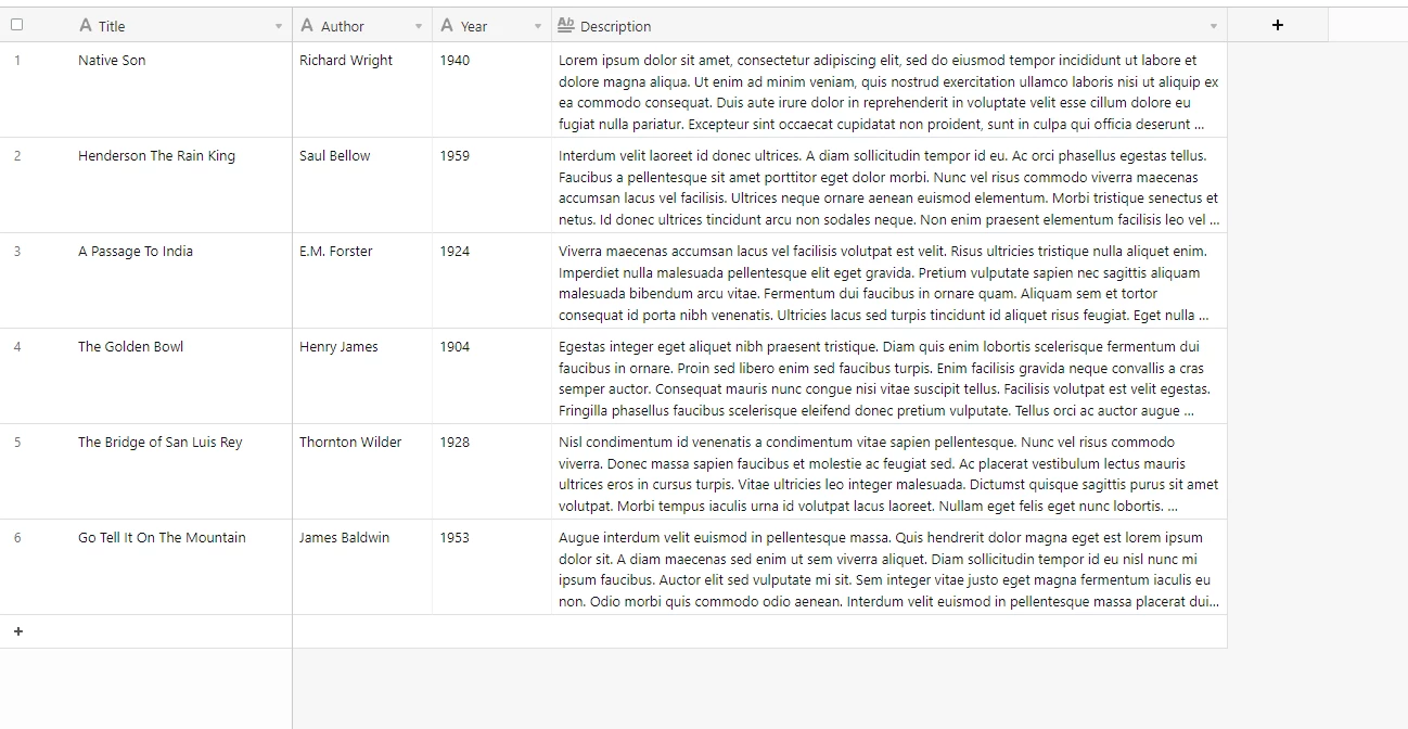
The thing is that I was already taking the “transform before you look” approach, but it didn’t work in pulling the Year into the rollup. In my Books table, I used this formula in the Entry field:
UPPER({Author}) & ". " & {Title} & ". " & {Place} & ": " & {Publisher} & ", " & “{Year}” & ". " & {Description} & " " & {Book Edition} & “. $” & {Price} & “.”
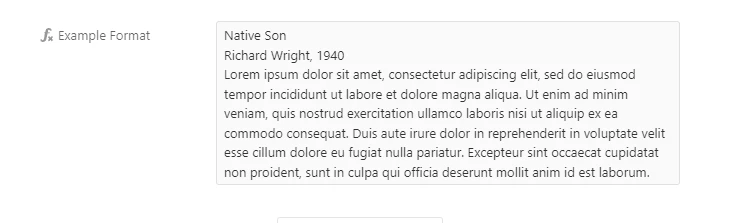
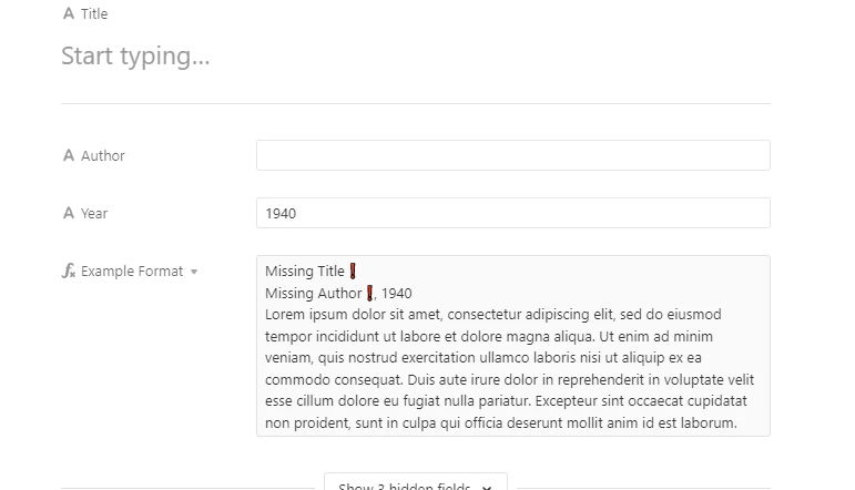
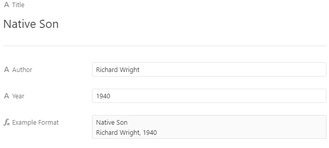
Even here, even in this formula field, even before the rollup field in the Catalogs table, {Year} stays {Year} and doesn’t give me the numbers. And the price is missing a digit. I’ll use your Native Son example, since I actually have one of those in my stock . . .
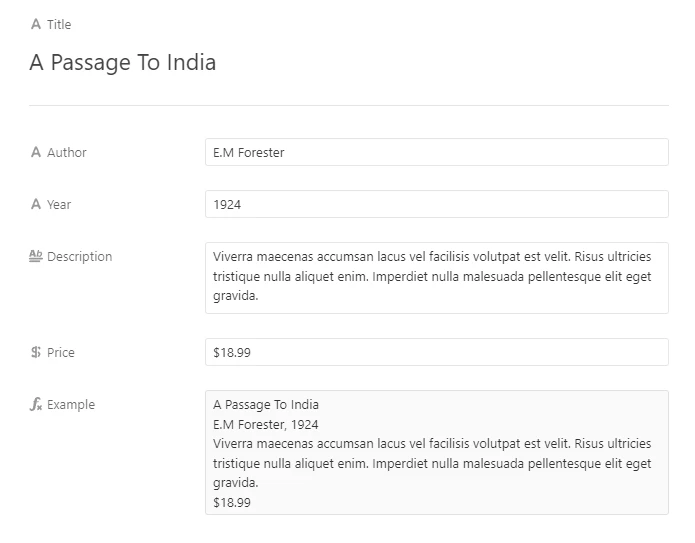
WRIGHT, RICHARD. Native Son. New York: Harper & Brothers, {Year}. A faithful facsimile of the first edition. First Edition Library prospectus laid in. Brand new, never read, and in a Brodart jacket cover. First Edition Facsimile. $41.5.
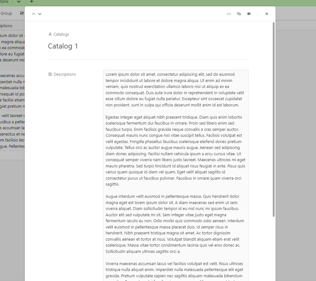
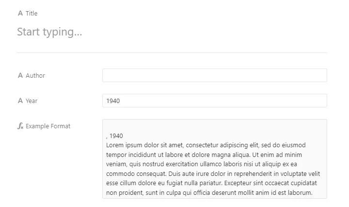
^ this is what the cell looks like in the Entry field of the Books table, before it’s pulled into the rollup field in the Catalogs table. Did I miss a step in your instructions on how to transform before you look?
Okay, let’s talk about this.
This is actually behaving as it should!
If you’re curious to read a bit about why this happens, you can read below.
Alternatively, if you want to skip to the solution, click here.
I could type out massive chunks to explain why this is the case, but I’ll provide you with some context.
Computers and programs interpret data in ‘types’. We literally call them data types.
For our purposes, here’s what we care about with Airtable’s formulas.
-
Booleans (True/False)
-
Strings (Text)
-
Numbers
-
Undefined (Literally nothing. Like forgetting the field even existed).
-
Date/Time (Not actually a data type, but for the sake of Airtable, we’ll toss it in).
Every field type in Airtable holds a certain type of data. (With the exceptions being the linked record and attachment fields, which use a type called an object.)
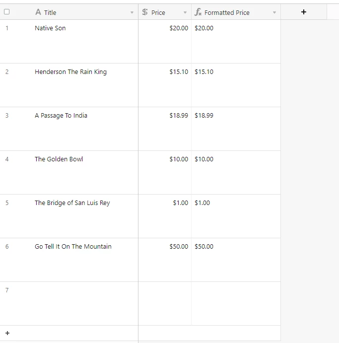
The currency field accepts numbers.
Despite being able to format data into a readable currency, Airtable only understands and interprets data in that field as being a number.
We see $20.00, but from Airtable’s perspective, it’s just 20.
This is, of course, quite simple.
However, it gets frustrating when we see $20.90 because Airtable sees 20.9.
So, how can we change this?
Well, since Airtable is looking at the currency field as a number (and thus doesn’t care about any formatting), we can take the number value and force Airtable to treat it as text.
Here’s a formula that will format numbers into a USD text format.
IF(
    {Price},
    IF(
        FIND(
            ".",
            {Price} & ""
        ),
        IF(
            REGEX_MATCH(
                {Price} & "",
                "\.[^0][^0]"
            ),
            "$" & {Price},
            IF(
                REGEX_MATCH(
                    {Price} & "",
                    "\.[^0]$"
                ),
                "$" & {Price} & "0"
            )
        ),
        "$" & {Price} & ".00"
    )
)
Here’s what the returned behavior looks like:
With this, you can correctly format numbers into a USD format within a text string inside a formula.
Here’s what the fully formatted, final output would look like using the original formula I posted:
REGEX_REPLACE(
    IF(
        {Title},
        TRIM({Title}) & "line"
    )
    &
    IF(
        {Author},
        TRIM({Author}) & IF(
            {Year},
            ", " & TRIM({Year}) & "line",
            "line"
        ),
        IF(
            {Year},
            TRIM({Year}) & "line"
        )
    )
    &
    IF(
        {Description},
        TRIM({Description}) & "line"
    )
    &
    IF(
        {Price},
        IF(
            FIND(
                ".",
                {Price} & ""
            ),
            IF(
                REGEX_MATCH(
                    {Price} & "",
                    "\.[^0][^0]"
                ),
                "$" & {Price},
                IF(
                    REGEX_MATCH(
                        {Price} & "",
                        "\.[^0]$"
                    ),
                    "$" & {Price} & "0"
                )
            ),
            "$" & {Price} & ".00"
        )
    ),
    "line",
    "\n"
)