- Airtable Community
- Discussions
- Ask A Question
- Formulas
- Re: Eliminating Commas Between Rollup Field Items
- Subscribe to RSS Feed
- Mark Topic as New
- Mark Topic as Read
- Float this Topic for Current User
- Bookmark
- Subscribe
- Mute
- Printer Friendly Page
Re: Eliminating Commas Between Rollup Field Items
- Mark as New
- Bookmark
- Subscribe
- Subscribe to RSS Feed
- Permalink
- Report Inappropriate Content
Aug 28, 2022 02:05 PM
Hi All,
I’m in the process of creating a catalog of related books that I can hopefully email out to customers, and, so far, that’s involved creating an Entries rollup field in my Catalogs table that pulls from my Books table using the ARRAYUNIQUE(values) aggregation formula. I did as much formatting as possible in the Books table, adding caps with UPPER() and spaces with \n, but I can’t figure out how to eliminate the comma after each rollup field item. I tried this:
SUBSTITUTE (ARRAYUNIQUE (values), “,”, " + ")
But I kept getting “Sorry, there was a problem saving this field. Please check your formula text.”
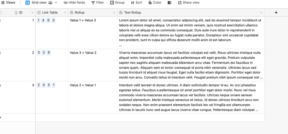
I’ll add a screenshot here so you can see what I’m talking about and why I’d want to eliminate the comma . . .
Thanks in advance for your suggestions!
Solved! Go to Solution.
Accepted Solutions
- Mark as New
- Bookmark
- Subscribe
- Subscribe to RSS Feed
- Permalink
- Report Inappropriate Content
Aug 29, 2022 09:32 AM
Okay, let’s talk about this.
This is actually behaving as it should!
If you’re curious to read a bit about why this happens, you can read below.
Alternatively, if you want to skip to the solution, click here.
I could type out massive chunks to explain why this is the case, but I’ll provide you with some context.
Computers and programs interpret data in ‘types’. We literally call them data types.
For our purposes, here’s what we care about with Airtable’s formulas.
-
Booleans (True/False)
-
Strings (Text)
-
Numbers
-
Undefined (Literally nothing. Like forgetting the field even existed).
-
Date/Time (Not actually a data type, but for the sake of Airtable, we’ll toss it in).
Every field type in Airtable holds a certain type of data. (With the exceptions being the linked record and attachment fields, which use a type called an object.)
The currency field accepts numbers.
Despite being able to format data into a readable currency, Airtable only understands and interprets data in that field as being a number.
We see $20.00, but from Airtable’s perspective, it’s just 20.
This is, of course, quite simple.
However, it gets frustrating when we see $20.90 because Airtable sees 20.9.
So, how can we change this?
Well, since Airtable is looking at the currency field as a number (and thus doesn’t care about any formatting), we can take the number value and force Airtable to treat it as text.
Here’s a formula that will format numbers into a USD text format.
IF(
    {Price},
    IF(
        FIND(
            ".",
            {Price} & ""
        ),
        IF(
            REGEX_MATCH(
                {Price} & "",
                "\.[^0][^0]"
            ),
            "$" & {Price},
            IF(
                REGEX_MATCH(
                    {Price} & "",
                    "\.[^0]$"
                ),
                "$" & {Price} & "0"
            )
        ),
        "$" & {Price} & ".00"
    )
)
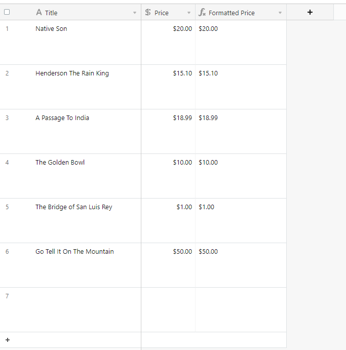
Here’s what the returned behavior looks like:
With this, you can correctly format numbers into a USD format within a text string inside a formula.
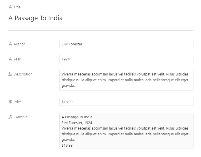
Here’s what the fully formatted, final output would look like using the original formula I posted:
REGEX_REPLACE(
    IF(
        {Title},
        TRIM({Title}) & "line"
    )
    &
    IF(
        {Author},
        TRIM({Author}) & IF(
            {Year},
            ", " & TRIM({Year}) & "line",
            "line"
        ),
        IF(
            {Year},
            TRIM({Year}) & "line"
        )
    )
    &
    IF(
        {Description},
        TRIM({Description}) & "line"
    )
    &
    IF(
        {Price},
        IF(
            FIND(
                ".",
                {Price} & ""
            ),
            IF(
                REGEX_MATCH(
                    {Price} & "",
                    "\.[^0][^0]"
                ),
                "$" & {Price},
                IF(
                    REGEX_MATCH(
                        {Price} & "",
                        "\.[^0]$"
                    ),
                    "$" & {Price} & "0"
                )
            ),
            "$" & {Price} & ".00"
        )
    ),
    "line",
    "\n"
)
- Mark as New
- Bookmark
- Subscribe
- Subscribe to RSS Feed
- Permalink
- Report Inappropriate Content
Aug 28, 2022 03:28 PM
Hey @Alba_Machado2!
Go ahead and try this formula and let me know if it works!
SUBSTITUTE(
    ARRAYUNIQUE(values),
    ",",
    " + "
)
- Mark as New
- Bookmark
- Subscribe
- Subscribe to RSS Feed
- Permalink
- Report Inappropriate Content
Aug 28, 2022 05:56 PM
Hi Ben!
Thanks for the suggestion, but, nope, it doesn’t work. It returns an ERROR to me. :confused:
- Mark as New
- Bookmark
- Subscribe
- Subscribe to RSS Feed
- Permalink
- Report Inappropriate Content
Aug 28, 2022 05:58 PM
Okay, one sec.
There isn’t a problem I cannot solve.
- Mark as New
- Bookmark
- Subscribe
- Subscribe to RSS Feed
- Permalink
- Report Inappropriate Content
Aug 28, 2022 06:11 PM
Boom.
IF(
    values,
    ARRAYJOIN(
        ARRAYUNIQUE(
            values
        ),
        ' + '
    )
)
Also, I just saw this:
You can also make these transformations within the rollup field without doing much in your other table.
Not too sure how you’re using the UPPER function, but here’s a quick example.
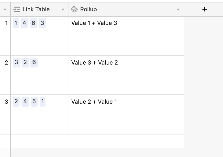
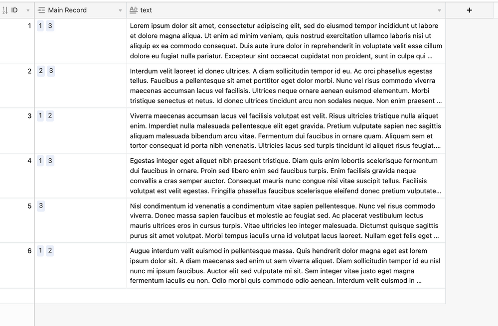
Here are my records with the text fields:
Here’s the table where I’m looking them up:
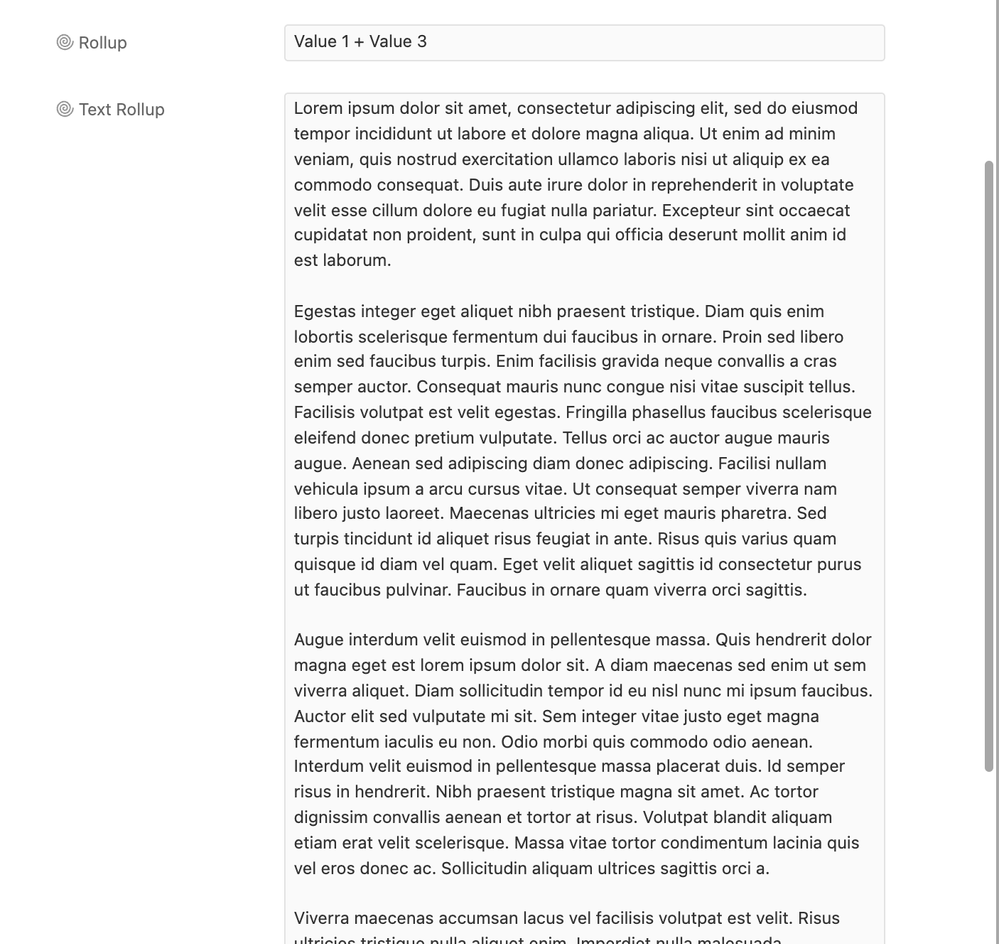
If I use this formula in the rollup field, I can automatically format and separate everything however I’d like:
IF(
    values,
    ARRAYJOIN(
        ARRAYUNIQUE(
            values
        ),
        '\n' & '\n'
    )
)
I apologize for the quick response!
I’m on my laptop and struggling without my main monitors.
Let me know if you have more that you’d like to do, or if you’re having trouble with any of it!
- Mark as New
- Bookmark
- Subscribe
- Subscribe to RSS Feed
- Permalink
- Report Inappropriate Content
Aug 28, 2022 06:33 PM
You did it! There really isn’t a problem you can’t solve! :open_mouth:
I was going to post new topics for a couple of other problems with this particular project, but since you offered so nicely…
For some reason, the Year is coming up as {Year} in the Entries rollup field. In the Books table, the Year field will say 1901. But in the Catalogs table’s Entries rollup field, I see {Year} instead.
And the one last problem is that the Price sometimes drops a digit. So, like, $31.50 will become $31.5.
Other than that, I’m pretty happy with the way this is working out and thrilled that you figured out how to solve the random comma problem. Thank you! Thank you! Thank you! :slightly_smiling_face:
- Mark as New
- Bookmark
- Subscribe
- Subscribe to RSS Feed
- Permalink
- Report Inappropriate Content
Aug 28, 2022 09:15 PM
Okay, there are a few things to cover.
First, let’s talk about the Year field.
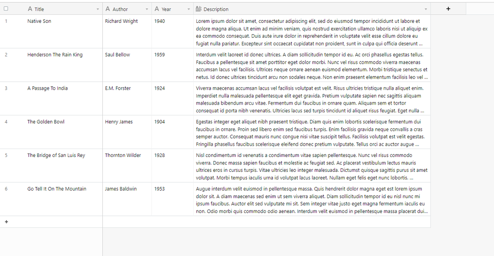
Let’s say this is your Books table:
We have the original text field that we were working with before.
Here, it’s the Description field.
I also added a Year field to hold the year of publication.
Let’s hop into our Catalogs table.
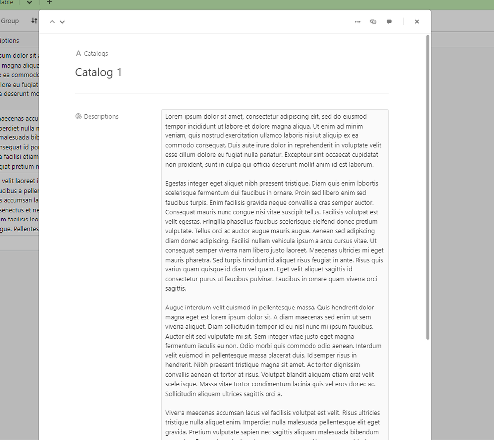
Here, we have the Description rollup field I previously walked you through.
We now want to get our publication year information into this rollup.
When trying to do this, we quickly encounter a huge deficiency in Airtable’s rollup & formula implementation.
When using Airtable’s rollups (or formulas that reference a linked record field), you cannot reference additional fields from a linked record.
So, if you’re trying to do this:
IF(
    AND(
        values,
        {Year}
    ARRAYJOIN(
        ARRAYUNIQUE(
            values
        ),
        '\n' & '\n'
    )
)
It won’t work, even if you’re referencing a valid field in another table. As far as Airtable is concerned, the object you’re trying to reference is just a text string.
Now we’re left sitting here asking ourselves what we can do next.
I think that are two ways to approach this scenario.
The first method is the way I would personally solve this.
After writing out this first method and starting the second one, I realized just how terrible the second method is. With that in mind, I’m not even going to try and describe the second method.
Leaving this info in to let you (and others) know there are a few ways to approach this puzzle. Not all solutions are worth your time.
Method 1: Transform Before You Look
You’ve actually done this, albeit in a slightly different way.
When using a rollup field, you take specific data from another source and then format it using formulas.
As we’ve just come to find, sometimes we don’t have as much flexibility as we need when doing this.
The solution with this method is to do all of our formatting before it ever touches our rollup.
This allows us to leverage all of the fields on the record and format it however we’d like without worrying about the limitations of the rollup field.
Here’s how…
This might vary for your requirements, but it’ll serve as an example.
To define what our final goal is, let’s say this will be our formatting goal:
{Title}
{Author}, {Year}
{Description}
It should look like this:
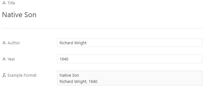
Native Son
Richard Wright, 1940
Lorem ipsum dolor sit amet, consectetur adipiscing elit, sed do eiusmod tempor incididunt ut labore et dolore magna aliqua.
Ut enim ad minim veniam, quis nostrud exercitation ullamco laboris nisi ut aliquip ex ea commodo consequat.
Here’s a formula that will meet these requirements:
{Title}
& "\n" &
{Author} & ", " & {Year}
& "\n" &
{Description}
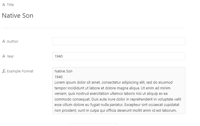
And here’s what that looks like:
Okay, dope.
We do, however, have a new problem.
What happens if one or more of these fields are blank?
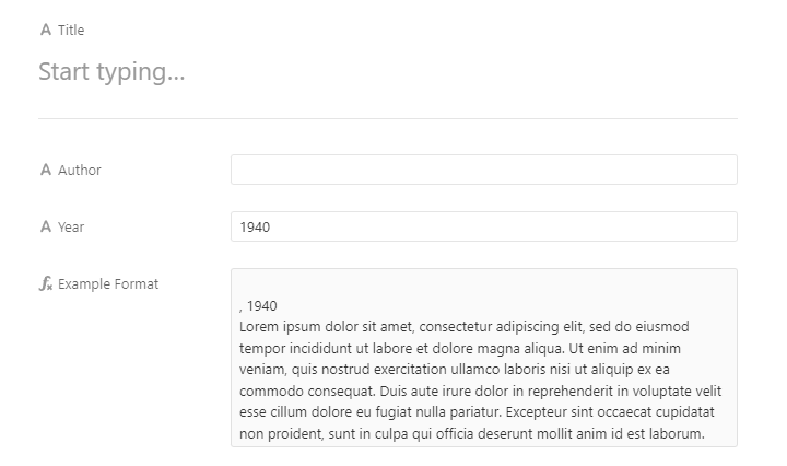
If I delete the Title and Author fields, it’ll give us this:
If you’re like me and hate this behavior, we’ll leverage nesting and a few tricks to account for these situations.
One way to do this is to create placeholders that will fill in for blank values.
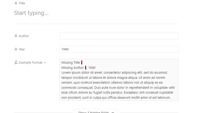
You’ll see this in this formula:
IF(
    {Title},
    {Title},
    "Missing Title ❗"
)
& "\n" &
IF(
    {Author},
    {Author},
    "Missing Author ❗" & ", "
)
&
IF(
    {Year},
    {Year},
    "Missing Year ❗"
)
& "\n" &
IF(
    {Description},
    {Description}
)
Here’s the formula field with this change:
This makes life a little bit easier.
The second way would be to make it fully dynamic. This means that the field will only fill in information it has and nothing else.
This is my preferred way since I am a bit picky about formatting.
REGEX_REPLACE(
    IF(
        {Title},
        TRIM({Title}) & "line"
    )
    &
    IF(
        {Author},
        TRIM({Author}) & IF(
            {Year},
            ", " & TRIM({Year}) & "line",
            "line"
        ),
        IF(
            {Year},
            TRIM({Year}) & "line"
        )
    )
    &
    IF(
        {Description},
        TRIM({Description}) & "line"
    ),
    "line",
    "\n"
)
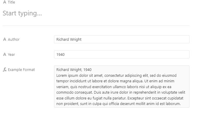
Here are some examples of the behavior that produces:
Okay, cool.
So what now?
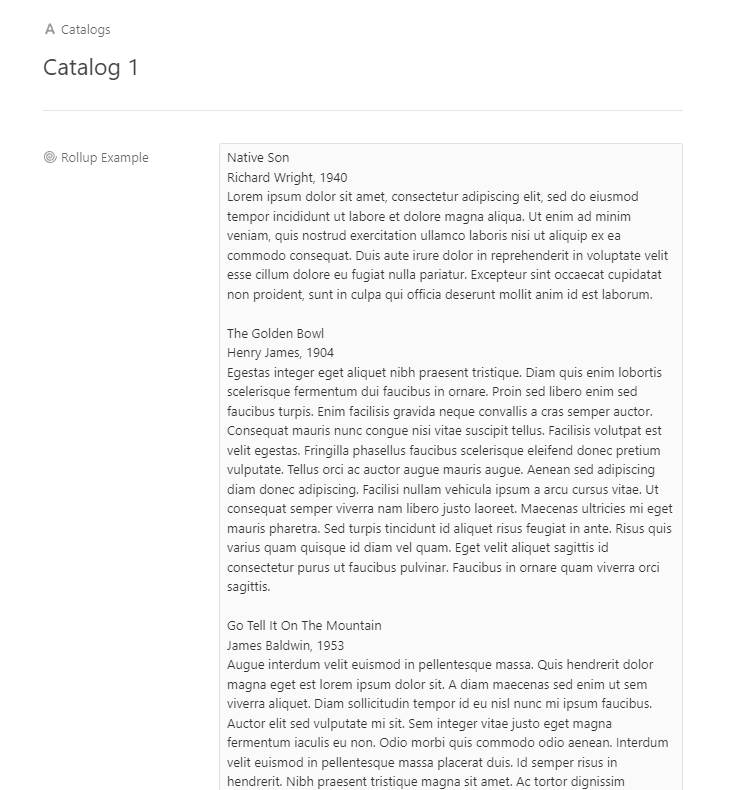
If you hop back into the Catalogs table and change the rollup field we created to point to the new formula field, it will provide you with the formatting we specified. Hence the method’s name, Transform Before You Look.
Here’s our end result:
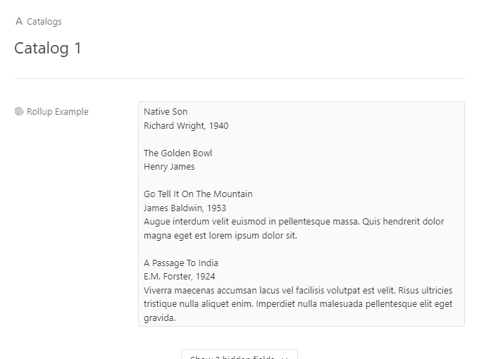
I trimmed some of the sample data to show a more reasonable example. Here’s what it (reasonably) looks like:
As you can see, even if data is missing, everything remains neatly formatted and clean.
I will type out the answer to the second part of your question regarding currency formatting.
Gimme a bit to get it out.
Edit:
8/19/2022: I realized that I didn’t quite like how the original formula worked. I changed the behavior of the formula to more accurately account for new line characters using a regex solution I put together a bit ago.
I did not update the screenshots since they still accurately represent the behavior of the new formula, as well as the previous one.
- Mark as New
- Bookmark
- Subscribe
- Subscribe to RSS Feed
- Permalink
- Report Inappropriate Content
Aug 28, 2022 10:18 PM
Wow, this is thorough. I still have to look into the trimming trick since, I, too, am picky about formatting—although less so with Airtable, since I’m not a pro like you.
The thing is that I was already taking the “transform before you look” approach, but it didn’t work in pulling the Year into the rollup. In my Books table, I used this formula in the Entry field:
UPPER({Author}) & ". " & {Title} & ". " & {Place} & ": " & {Publisher} & ", " & “{Year}” & ". " & {Description} & " " & {Book Edition} & “. $” & {Price} & “.”
Even here, even in this formula field, even before the rollup field in the Catalogs table, {Year} stays {Year} and doesn’t give me the numbers. And the price is missing a digit. I’ll use your Native Son example, since I actually have one of those in my stock . . .
WRIGHT, RICHARD. Native Son. New York: Harper & Brothers, {Year}. A faithful facsimile of the first edition. First Edition Library prospectus laid in. Brand new, never read, and in a Brodart jacket cover. First Edition Facsimile. $41.5.
^ this is what the cell looks like in the Entry field of the Books table, before it’s pulled into the rollup field in the Catalogs table. Did I miss a step in your instructions on how to transform before you look?
- Mark as New
- Bookmark
- Subscribe
- Subscribe to RSS Feed
- Permalink
- Report Inappropriate Content
Aug 29, 2022 08:02 AM
Try this:
UPPER(
    {Author}
) & ". " & {Title} & ". " & {Place} & ": " & {Publisher} & ", " & {Year} & ". " & {Description} & " " & {Book Edition} & ". $" & {Price} & "."
- Mark as New
- Bookmark
- Subscribe
- Subscribe to RSS Feed
- Permalink
- Report Inappropriate Content
Aug 29, 2022 09:32 AM
Okay, let’s talk about this.
This is actually behaving as it should!
If you’re curious to read a bit about why this happens, you can read below.
Alternatively, if you want to skip to the solution, click here.
I could type out massive chunks to explain why this is the case, but I’ll provide you with some context.
Computers and programs interpret data in ‘types’. We literally call them data types.
For our purposes, here’s what we care about with Airtable’s formulas.
-
Booleans (True/False)
-
Strings (Text)
-
Numbers
-
Undefined (Literally nothing. Like forgetting the field even existed).
-
Date/Time (Not actually a data type, but for the sake of Airtable, we’ll toss it in).
Every field type in Airtable holds a certain type of data. (With the exceptions being the linked record and attachment fields, which use a type called an object.)
The currency field accepts numbers.
Despite being able to format data into a readable currency, Airtable only understands and interprets data in that field as being a number.
We see $20.00, but from Airtable’s perspective, it’s just 20.
This is, of course, quite simple.
However, it gets frustrating when we see $20.90 because Airtable sees 20.9.
So, how can we change this?
Well, since Airtable is looking at the currency field as a number (and thus doesn’t care about any formatting), we can take the number value and force Airtable to treat it as text.
Here’s a formula that will format numbers into a USD text format.
IF(
    {Price},
    IF(
        FIND(
            ".",
            {Price} & ""
        ),
        IF(
            REGEX_MATCH(
                {Price} & "",
                "\.[^0][^0]"
            ),
            "$" & {Price},
            IF(
                REGEX_MATCH(
                    {Price} & "",
                    "\.[^0]$"
                ),
                "$" & {Price} & "0"
            )
        ),
        "$" & {Price} & ".00"
    )
)
Here’s what the returned behavior looks like:
With this, you can correctly format numbers into a USD format within a text string inside a formula.
Here’s what the fully formatted, final output would look like using the original formula I posted:
REGEX_REPLACE(
    IF(
        {Title},
        TRIM({Title}) & "line"
    )
    &
    IF(
        {Author},
        TRIM({Author}) & IF(
            {Year},
            ", " & TRIM({Year}) & "line",
            "line"
        ),
        IF(
            {Year},
            TRIM({Year}) & "line"
        )
    )
    &
    IF(
        {Description},
        TRIM({Description}) & "line"
    )
    &
    IF(
        {Price},
        IF(
            FIND(
                ".",
                {Price} & ""
            ),
            IF(
                REGEX_MATCH(
                    {Price} & "",
                    "\.[^0][^0]"
                ),
                "$" & {Price},
                IF(
                    REGEX_MATCH(
                        {Price} & "",
                        "\.[^0]$"
                    ),
                    "$" & {Price} & "0"
                )
            ),
            "$" & {Price} & ".00"
        )
    ),
    "line",
    "\n"
)
